##
! {RMODFLOW} is still in its experimental lifecycle stage.
##
! Use at your own risk, and submit issues here:
##
! <https://github.com/rogiersbart/RMODFLOW/issues>
A MODFLOW simulation can create multiple output files representing different variables. Examples are hydraulic heads (hed), drawdowns (ddn), cell-by-cell flow files (cbc), head-prediction files (hpr) and the listing file. The latter holds information on the simulation, execution and solver progress and a volumetric budget if defined by the Output-Control file (OC). This budget (bud) is often useful to look at.
These files can be written by MODFLOW in a variety of types and formats such as binary or ASCII. The internal structure of those files can also take various forms. RMODFLOW can handle all those formats, even the more obscure ones. In most cases, you’ll only need to supply a dis object to the rmf_read_* function. If the file is binary, you’ll need to know if it’s single or double precision depending on which MODFLOW executable was used. Most of the time, this would have been single precision.
Heads & drawdowns
To read simulated heads, use rmf_read_hed() (or its alias, rmf_read_head()). By default, binary = TRUE and precision = 'single'. If either of those arguments are incorrect, RMODFLOW will throw an error and suggests changing them. You can also supply a bas object to remove no-flow values or supply a hdry vector with values to set to NA.
dis <- rmf_example_file("water-supply-problem.dis") %>%
  rmf_read_dis()

head <- rmf_example_file("water-supply-problem.fhd") %>%
  rmf_read_hed(dis = dis, binary = FALSE)
Drawdowns are similar to heads; use rmf_read_ddn() or its alias rmf_read_drawdown().
ddn <- rmf_example_file("water-supply-problem.fdn") %>%
  rmf_read_ddn(dis = dis, binary = FALSE)
Heads and drawdowns are objects of class hed and ddn, respectively. Additionally, they are rmf_4d_arrays. Besides the default rmf_array attributes, these objects also have additional attributes related to the timing of each time step in the 4th dimensions of the array:
str(head)
#>  'hed' num [1:45, 1:56, 1, 1:16] -1e+20 -1e+20 -1e+20 -1e+20 -1e+20 ...
#>  - attr(*, "nstp")= num [1:16] 1 2 3 4 5 6 7 8 9 10 ...
#>  - attr(*, "totim")= num [1:16] 293 707 1293 2121 3292 ...
#>  - attr(*, "pertim")= num [1:16] 293 707 1293 2121 3292 ...
#>  - attr(*, "kper")= num [1:16] 1 1 1 1 1 1 1 1 1 1 ...
#>  - attr(*, "kstp")= num [1:16] 1 2 3 4 5 6 7 8 9 10 ...
#>  - attr(*, "dimlabels")= chr [1:4] "i" "j" "k" "l"
To only read in certain time-steps, use the timesteps argument:
rmf_example_file("water-supply-problem.fhd") %>%
  rmf_read_hed(dis = dis, binary = FALSE, timesteps = c(1,16)) %>%
  str()
#>  'hed' num [1:45, 1:56, 1, 1:2] -1e+20 -1e+20 -1e+20 -1e+20 -1e+20 ...
#>  - attr(*, "nstp")= num [1:2] 1 16
#>  - attr(*, "totim")= num [1:2] 293 180000
#>  - attr(*, "pertim")= num [1:2] 293 180000
#>  - attr(*, "kper")= num [1:2] 1 1
#>  - attr(*, "kstp")= num [1:2] 1 16
#>  - attr(*, "dimlabels")= chr [1:4] "i" "j" "k" "l"
RMODFLOW provides S3 plotting methods for hed and ddn objects which act as wrappers for rmf_plot.rmf_4d_array():
# read bas to remove no-flow values from plot.
# Alternatively, this could have been done by supplying a bas object to rmf_read_hed
bas <- rmf_example_file("water-supply-problem.bas") %>%
  rmf_read_bas(dis = dis)

rmf_plot(head, dis = dis, bas = bas, k = 1)
#> Warning: Plotting final time step results.
By default, the last time step is plotted. As with rmf_plot.rmf_4d_array, you can specify the l argument to subset the 4th dimension directly. Alternatively for hed, ddn and cbc objects, you can supply a kper and kstp argument to the respective rmf_plot call. For hed & ddn, you can also supply the absolute time step number using nstp:
rmf_plot(head, dis = dis, bas = bas, k = 1, kper = 1, kstp = 16)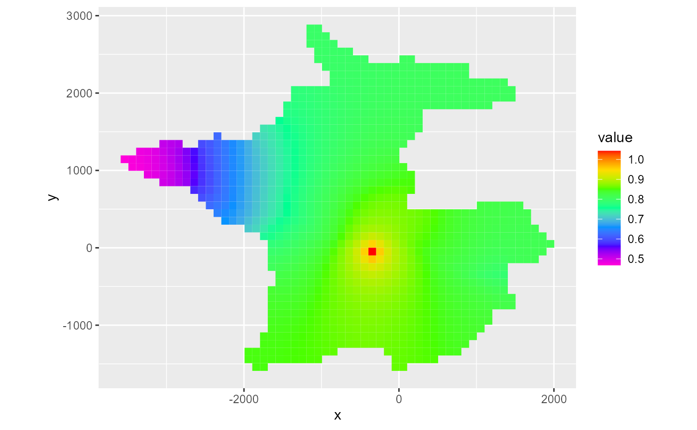
rmf_plot(head, dis = dis, bas = bas, k = 1, nstp = 12)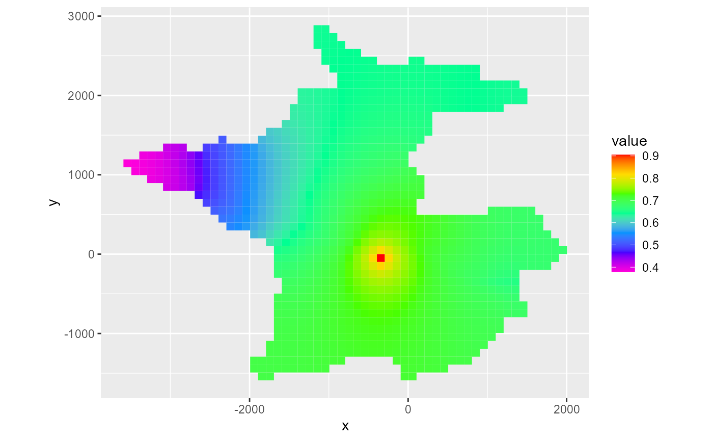
When plotting a hed object, a saturated argument can be supplied. By default, this is set to TRUE, which plots the saturated part of the grid when a cross-section plot is made. This can be useful if the potentiometric surface needs to be displayed. If set to FALSE, the cells are completely filled.
m <- rmf_example_file('rocky-mountain-arsenal.nam') %>%
  rmf_read(output = TRUE, verbose = FALSE)

rmf_plot(m$head, dis = m$dis, bas = m$bas, j = 25, grid = TRUE, saturated = TRUE) # default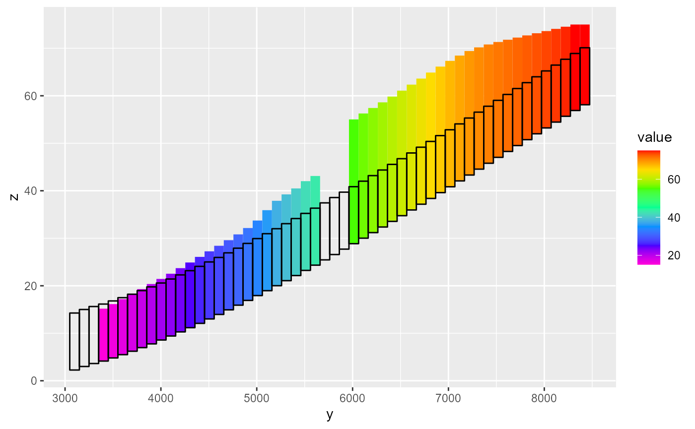
rmf_plot(m$head, dis = m$dis, bas = m$bas, j = 25, grid = TRUE, saturated = FALSE)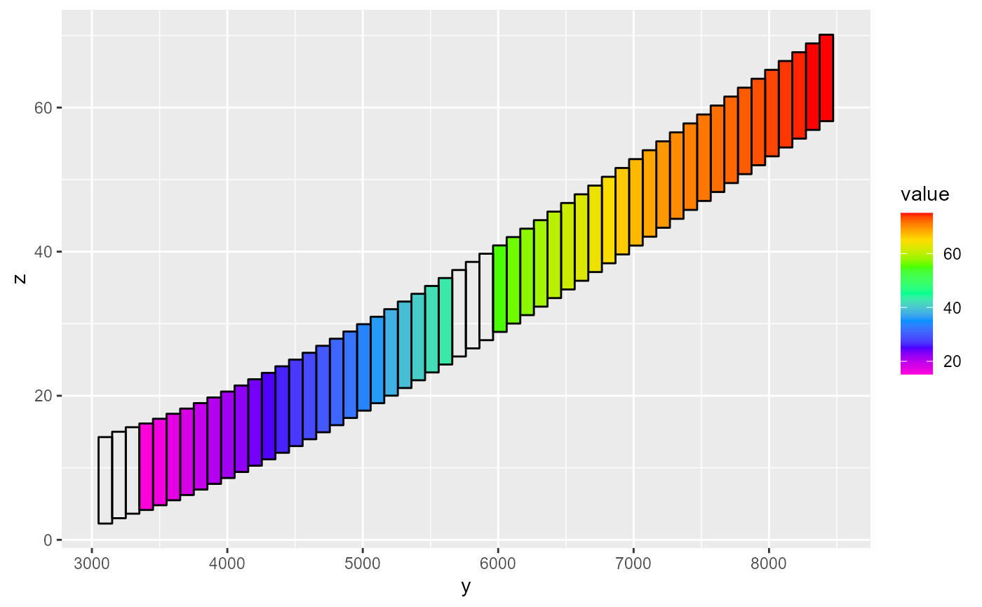
It does not affect the mapview plot however:
# same results
rmf_plot(m$head, dis = m$dis, bas = m$bas, k = 1, saturated = TRUE) # default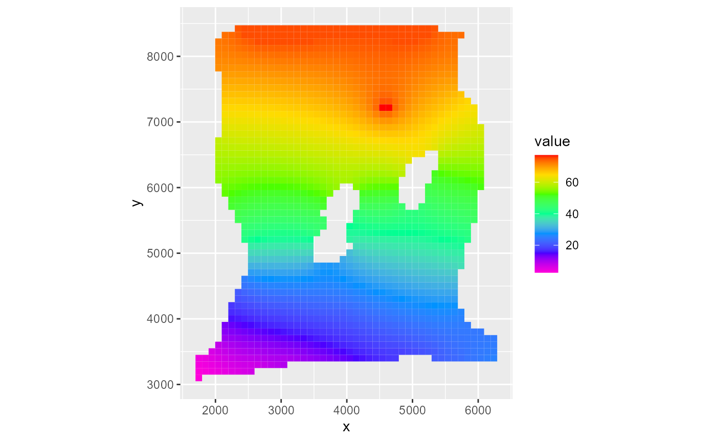
rmf_plot(m$head, dis = m$dis, bas = m$bas, k = 1, saturated = FALSE)
We can obtain a water-table surface from the hed object using rmf_convert_hed_to_water_table which returns a rmf_2d_array, which also takes an l argument to subset the time step of the hed object (by default takes the last time step):
wt <- rmf_convert_hed_to_water_table(head, l = 10)
str(wt)
#>  'rmf_2d_array' num [1:45, 1:56] -1e+20 -1e+20 -1e+20 -1e+20 -1e+20 ...
#>  - attr(*, "dimlabels")= chr [1:2] "i" "j"
Cell-by-cell flow budget
A cbc file is always binary. Reading in such a file can be done by using the rmf_read_cbc() function which returns a list with flow components, which are either rmf_list objects or rmf_4d_array objects.
cbc <- rmf_example_file("water-supply-problem.cbc") %>%
  rmf_read_cbc(dis = dis)
str(cbc)
#> List of 5
#>  $ storage        : 'rmf_4d_array' num [1:45, 1:56, 1, 1:16] 0 0 0 0 0 0 0 0 0 0 ...
#>   ..- attr(*, "dimlabels")= chr [1:4] "i" "j" "k" "l"
#>   ..- attr(*, "nstp")= int [1:16] 1 2 3 4 5 6 7 8 9 10 ...
#>   ..- attr(*, "delt")= num [1:16] 293 414 586 828 1171 ...
#>   ..- attr(*, "totim")= num [1:16] 293 707 1293 2121 3292 ...
#>   ..- attr(*, "pertim")= num [1:16] 293 707 1293 2121 3292 ...
#>   ..- attr(*, "kper")= int [1:16] 1 1 1 1 1 1 1 1 1 1 ...
#>   ..- attr(*, "kstp")= int [1:16] 1 2 3 4 5 6 7 8 9 10 ...
#>  $ flow_right_face: 'rmf_4d_array' num [1:45, 1:56, 1, 1:16] 0 0 0 0 0 0 0 0 0 0 ...
#>   ..- attr(*, "dimlabels")= chr [1:4] "i" "j" "k" "l"
#>   ..- attr(*, "nstp")= int [1:16] 1 2 3 4 5 6 7 8 9 10 ...
#>   ..- attr(*, "delt")= num [1:16] 293 414 586 828 1171 ...
#>   ..- attr(*, "totim")= num [1:16] 293 707 1293 2121 3292 ...
#>   ..- attr(*, "pertim")= num [1:16] 293 707 1293 2121 3292 ...
#>   ..- attr(*, "kper")= int [1:16] 1 1 1 1 1 1 1 1 1 1 ...
#>   ..- attr(*, "kstp")= int [1:16] 1 2 3 4 5 6 7 8 9 10 ...
#>  $ flow_front_face: 'rmf_4d_array' num [1:45, 1:56, 1, 1:16] 0 0 0 0 0 0 0 0 0 0 ...
#>   ..- attr(*, "dimlabels")= chr [1:4] "i" "j" "k" "l"
#>   ..- attr(*, "nstp")= int [1:16] 1 2 3 4 5 6 7 8 9 10 ...
#>   ..- attr(*, "delt")= num [1:16] 293 414 586 828 1171 ...
#>   ..- attr(*, "totim")= num [1:16] 293 707 1293 2121 3292 ...
#>   ..- attr(*, "pertim")= num [1:16] 293 707 1293 2121 3292 ...
#>   ..- attr(*, "kper")= int [1:16] 1 1 1 1 1 1 1 1 1 1 ...
#>   ..- attr(*, "kstp")= int [1:16] 1 2 3 4 5 6 7 8 9 10 ...
#>  $ wells          :Classes 'rmf_list' and 'data.frame':  16 obs. of  8 variables:
#>   ..$ k    : num [1:16] 1 1 1 1 1 1 1 1 1 1 ...
#>   ..$ i    : num [1:16] 30 30 30 30 30 30 30 30 30 30 ...
#>   ..$ j    : num [1:16] 33 33 33 33 33 33 33 33 33 33 ...
#>   ..$ value: num [1:16] 0.963 0.963 0.963 0.963 0.963 ...
#>   ..$ iface: num [1:16] 0 0 0 0 0 0 0 0 0 0 ...
#>   ..$ nstp : int [1:16] 1 2 3 4 5 6 7 8 9 10 ...
#>   ..$ kper : int [1:16] 1 1 1 1 1 1 1 1 1 1 ...
#>   ..$ kstp : int [1:16] 1 2 3 4 5 6 7 8 9 10 ...
#>   ..- attr(*, "kstp")= int [1:16] 1 2 3 4 5 6 7 8 9 10 ...
#>   ..- attr(*, "kper")= int [1:16] 1 1 1 1 1 1 1 1 1 1 ...
#>   ..- attr(*, "nstp")= int [1:16] 1 2 3 4 5 6 7 8 9 10 ...
#>   ..- attr(*, "pertim")= num [1:16] 293 707 1293 2121 3292 ...
#>   ..- attr(*, "totim")= num [1:16] 293 707 1293 2121 3292 ...
#>   ..- attr(*, "delt")= num [1:16] 293 414 586 828 1171 ...
#>   ..- attr(*, "ctmp")=List of 16
#>   .. ..$ : chr "iface"
#>   .. ..$ : chr "iface"
#>   .. ..$ : chr "iface"
#>   .. ..$ : chr "iface"
#>   .. ..$ : chr "iface"
#>   .. ..$ : chr "iface"
#>   .. ..$ : chr "iface"
#>   .. ..$ : chr "iface"
#>   .. ..$ : chr "iface"
#>   .. ..$ : chr "iface"
#>   .. ..$ : chr "iface"
#>   .. ..$ : chr "iface"
#>   .. ..$ : chr "iface"
#>   .. ..$ : chr "iface"
#>   .. ..$ : chr "iface"
#>   .. ..$ : chr "iface"
#>  $ river_leakage  :Classes 'rmf_list' and 'data.frame':  1072 obs. of  8 variables:
#>   ..$ k    : num [1:1072] 1 1 1 1 1 1 1 1 1 1 ...
#>   ..$ i    : num [1:1072] 18 19 19 19 19 20 20 20 21 21 ...
#>   ..$ j    : num [1:1072] 1 1 2 3 4 4 5 6 6 7 ...
#>   ..$ value: num [1:1072] -1.07e-06 0.00 -1.17e-06 -1.27e-06 -1.46e-06 ...
#>   ..$ iface: num [1:1072] 0 0 0 0 0 0 0 0 0 0 ...
#>   ..$ nstp : int [1:1072] 1 1 1 1 1 1 1 1 1 1 ...
#>   ..$ kper : int [1:1072] 1 1 1 1 1 1 1 1 1 1 ...
#>   ..$ kstp : int [1:1072] 1 1 1 1 1 1 1 1 1 1 ...
#>   ..- attr(*, "kstp")= int [1:16] 1 2 3 4 5 6 7 8 9 10 ...
#>   ..- attr(*, "kper")= int [1:16] 1 1 1 1 1 1 1 1 1 1 ...
#>   ..- attr(*, "nstp")= int [1:16] 1 2 3 4 5 6 7 8 9 10 ...
#>   ..- attr(*, "pertim")= num [1:16] 293 707 1293 2121 3292 ...
#>   ..- attr(*, "totim")= num [1:16] 293 707 1293 2121 3292 ...
#>   ..- attr(*, "delt")= num [1:16] 293 414 586 828 1171 ...
#>   ..- attr(*, "ctmp")=List of 16
#>   .. ..$ : chr "iface"
#>   .. ..$ : chr "iface"
#>   .. ..$ : chr "iface"
#>   .. ..$ : chr "iface"
#>   .. ..$ : chr "iface"
#>   .. ..$ : chr "iface"
#>   .. ..$ : chr "iface"
#>   .. ..$ : chr "iface"
#>   .. ..$ : chr "iface"
#>   .. ..$ : chr "iface"
#>   .. ..$ : chr "iface"
#>   .. ..$ : chr "iface"
#>   .. ..$ : chr "iface"
#>   .. ..$ : chr "iface"
#>   .. ..$ : chr "iface"
#>   .. ..$ : chr "iface"
#>  - attr(*, "class")= chr "cbc"
A fluxes argument can be specified to only read in certain fluxes (see help(rmf_read_cbc) for details on which fluxes can be read). By default, all fluxes are read.
rmf_example_file("water-supply-problem.cbc") %>%
  rmf_read_cbc(dis = dis, fluxes = c("wells", "flow_right_face")) %>%
  str()
#> List of 2
#>  $ flow_right_face: 'rmf_4d_array' num [1:45, 1:56, 1, 1:16] 0 0 0 0 0 0 0 0 0 0 ...
#>   ..- attr(*, "dimlabels")= chr [1:4] "i" "j" "k" "l"
#>   ..- attr(*, "nstp")= int [1:16] 1 2 3 4 5 6 7 8 9 10 ...
#>   ..- attr(*, "delt")= num [1:16] 293 414 586 828 1171 ...
#>   ..- attr(*, "totim")= num [1:16] 293 707 1293 2121 3292 ...
#>   ..- attr(*, "pertim")= num [1:16] 293 707 1293 2121 3292 ...
#>   ..- attr(*, "kper")= int [1:16] 1 1 1 1 1 1 1 1 1 1 ...
#>   ..- attr(*, "kstp")= int [1:16] 1 2 3 4 5 6 7 8 9 10 ...
#>  $ wells          :Classes 'rmf_list' and 'data.frame':  16 obs. of  8 variables:
#>   ..$ k    : num [1:16] 1 1 1 1 1 1 1 1 1 1 ...
#>   ..$ i    : num [1:16] 30 30 30 30 30 30 30 30 30 30 ...
#>   ..$ j    : num [1:16] 33 33 33 33 33 33 33 33 33 33 ...
#>   ..$ value: num [1:16] 0.963 0.963 0.963 0.963 0.963 ...
#>   ..$ iface: num [1:16] 0 0 0 0 0 0 0 0 0 0 ...
#>   ..$ nstp : int [1:16] 1 2 3 4 5 6 7 8 9 10 ...
#>   ..$ kper : int [1:16] 1 1 1 1 1 1 1 1 1 1 ...
#>   ..$ kstp : int [1:16] 1 2 3 4 5 6 7 8 9 10 ...
#>   ..- attr(*, "kstp")= int [1:16] 1 2 3 4 5 6 7 8 9 10 ...
#>   ..- attr(*, "kper")= int [1:16] 1 1 1 1 1 1 1 1 1 1 ...
#>   ..- attr(*, "nstp")= int [1:16] 1 2 3 4 5 6 7 8 9 10 ...
#>   ..- attr(*, "pertim")= num [1:16] 293 707 1293 2121 3292 ...
#>   ..- attr(*, "totim")= num [1:16] 293 707 1293 2121 3292 ...
#>   ..- attr(*, "delt")= num [1:16] 293 414 586 828 1171 ...
#>   ..- attr(*, "ctmp")=List of 16
#>   .. ..$ : chr "iface"
#>   .. ..$ : chr "iface"
#>   .. ..$ : chr "iface"
#>   .. ..$ : chr "iface"
#>   .. ..$ : chr "iface"
#>   .. ..$ : chr "iface"
#>   .. ..$ : chr "iface"
#>   .. ..$ : chr "iface"
#>   .. ..$ : chr "iface"
#>   .. ..$ : chr "iface"
#>   .. ..$ : chr "iface"
#>   .. ..$ : chr "iface"
#>   .. ..$ : chr "iface"
#>   .. ..$ : chr "iface"
#>   .. ..$ : chr "iface"
#>   .. ..$ : chr "iface"
#>  - attr(*, "class")= chr "cbc"
Similar to heads and drawdowns, RMODFLOW has a rmf_plot.cbc() function which acts as a wrapper around either rmf_plot.rmf_list() or rmf_plot.rmf_4d_array() depending on which flux component to plot as defined by the flux argument:
rmf_plot(cbc, dis = dis, bas = bas, k = 1, flux = "storage")
#> Warning: Plotting final time step results.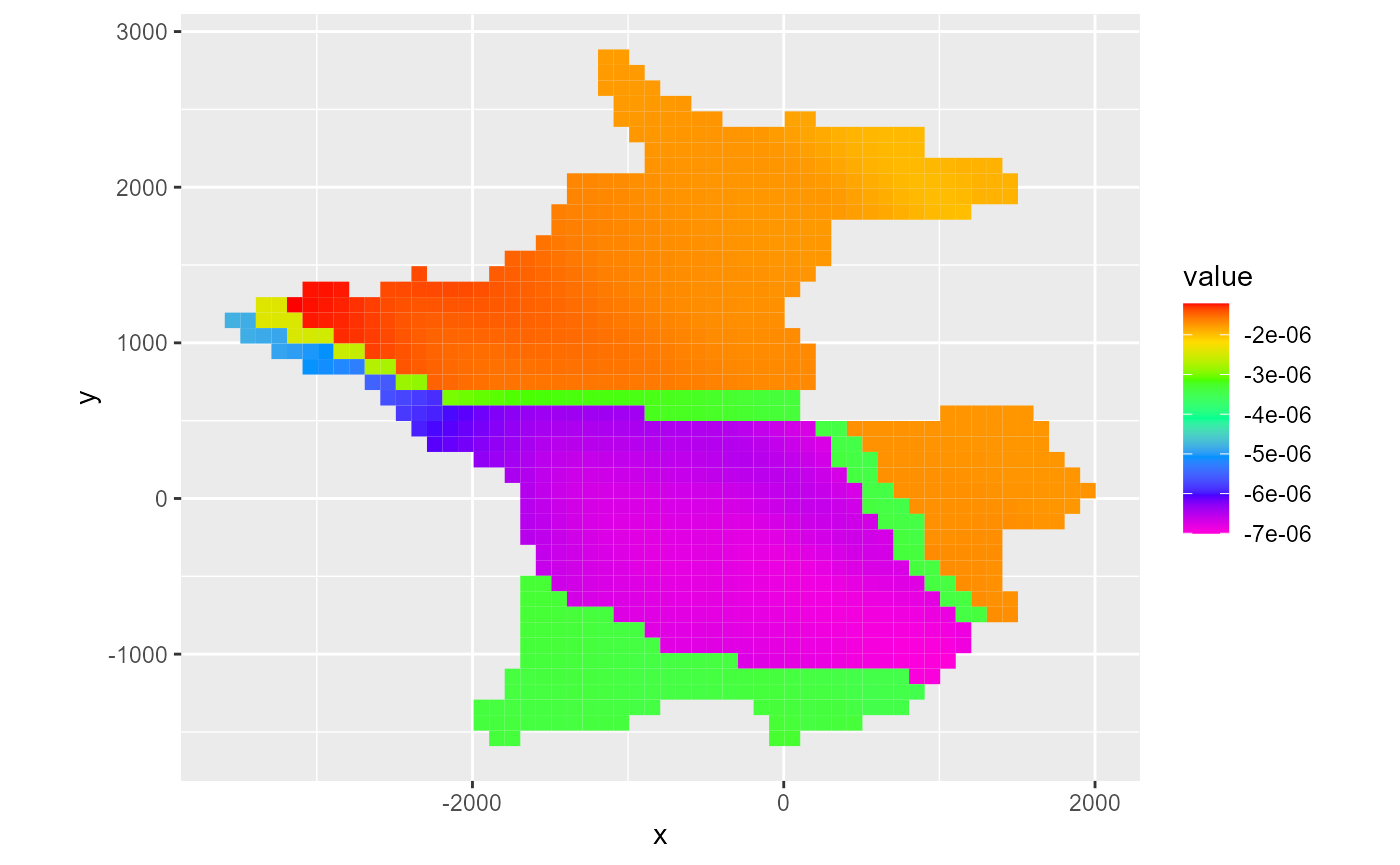
rmf_plot(cbc, dis = dis, bas = bas, k = 1, flux = "river_leakage")
#> Warning: Plotting final time step results.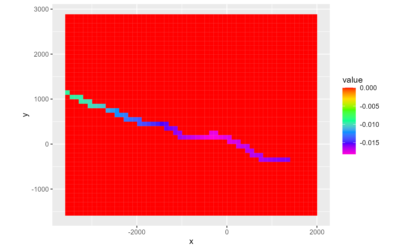
In addition to the available fluxes in the cbc object, the flux argument can also be darcy which will calculate Darcy fluxes using rmf_convert_cbc_to_darcy(). This is useful in conjunction with the type = 'vector' argument:
rmf_plot(head, dis = dis, bas = bas, k = 1, l = 16) +
  rmf_plot(cbc, dis = dis, bas = bas, k = 1, l = 16, flux = "darcy", type = "vector", add = TRUE)
#> Warning: Removed 1537 rows containing non-finite values (stat_quiver).
Volumetric budget
Useful as the cbc object may be, it is not always straightforward to obtain a mass balance (i.e. volumetric budget) from it. This is written to the listing file if specified by the OC file. To read in the volumetric budget from a listing file, use rmf_read_bud() which returns a bud object which is a list with two data.frames: one holding the volumetric rates and one with the cumulative volumes. Note: in previous versions of RMODFLOW, rmf_read_bud was used to read in the cell-by-cell flow object; this is therefore a breaking change:
bud <- rmf_example_file("water-supply-problem.lst") %>%
rmf_read_bud()
str(bud)
#> List of 2
#> $ cumulative:'data.frame': 16 obs. of 14 variables:
#> ..$ kstp : num [1:16] 1 2 3 4 5 6 7 8 9 10 ...
#> ..$ kper : num [1:16] 1 1 1 1 1 1 1 1 1 1 ...
#> ..$ storage_in : num [1:16] 0 0 0 0 0 0 0 0 0 0 ...
#> ..$ constant_head_in : num [1:16] 0 0 0 0 0 0 0 0 0 0 ...
#> ..$ wells_in : num [1:16] 282 681 1245 2043 3170 ...
#> ..$ river_leakage_in : num [1:16] 0 0 0 0 0 0 0 0 0 0 ...
#> ..$ total_in : num [1:16] 282 681 1245 2043 3170 ...
#> ..$ storage_out : num [1:16] 277 662 1192 1914 2884 ...
#> ..$ constant_head_out: num [1:16] 0 0 0 0 0 0 0 0 0 0 ...
#> ..$ wells_out : num [1:16] 0 0 0 0 0 0 0 0 0 0 ...
#> ..$ river_leakage_out: num [1:16] 4.47 18.51 52.42 127.17 284.2 ...
#> ..$ total_out : num [1:16] 282 680 1244 2041 3169 ...
#> ..$ difference : num [1:16] 0.309 0.695 1.049 1.455 1.732 ...
#> ..$ discrepancy : num [1:16] 0.11 0.1 0.08 0.07 0.05 0.04 0.03 0.03 0.02 0.02 ...
#> $ rates :'data.frame': 16 obs. of 14 variables:
#> ..$ kstp : num [1:16] 1 2 3 4 5 6 7 8 9 10 ...
#> ..$ kper : num [1:16] 1 1 1 1 1 1 1 1 1 1 ...
#> ..$ storage_in : num [1:16] 0 0 0 0 0 0 0 0 0 0 ...
#> ..$ constant_head_in : num [1:16] 0 0 0 0 0 0 0 0 0 0 ...
#> ..$ wells_in : num [1:16] 0.963 0.963 0.963 0.963 0.963 0.963 0.963 0.963 0.963 0.963 ...
#> ..$ river_leakage_in : num [1:16] 0 0 0 0 0 0 0 0 0 0 ...
#> ..$ total_in : num [1:16] 0.963 0.963 0.963 0.963 0.963 0.963 0.963 0.963 0.963 0.963 ...
#> ..$ storage_out : num [1:16] 0.947 0.928 0.904 0.872 0.829 ...
#> ..$ constant_head_out: num [1:16] 0 0 0 0 0 0 0 0 0 0 ...
#> ..$ wells_out : num [1:16] 0 0 0 0 0 0 0 0 0 0 ...
#> ..$ river_leakage_out: num [1:16] 0.0153 0.0339 0.0579 0.0902 0.1341 ...
#> ..$ total_out : num [1:16] 0.962 0.962 0.962 0.963 0.963 ...
#> ..$ difference : num [1:16] 0.001054 0.000932 0.000605 0.000489 0.000237 ...
#> ..$ discrepancy : num [1:16] 0.11 0.1 0.06 0.05 0.02 0.02 0.01 0.01 0.01 0.02 ...
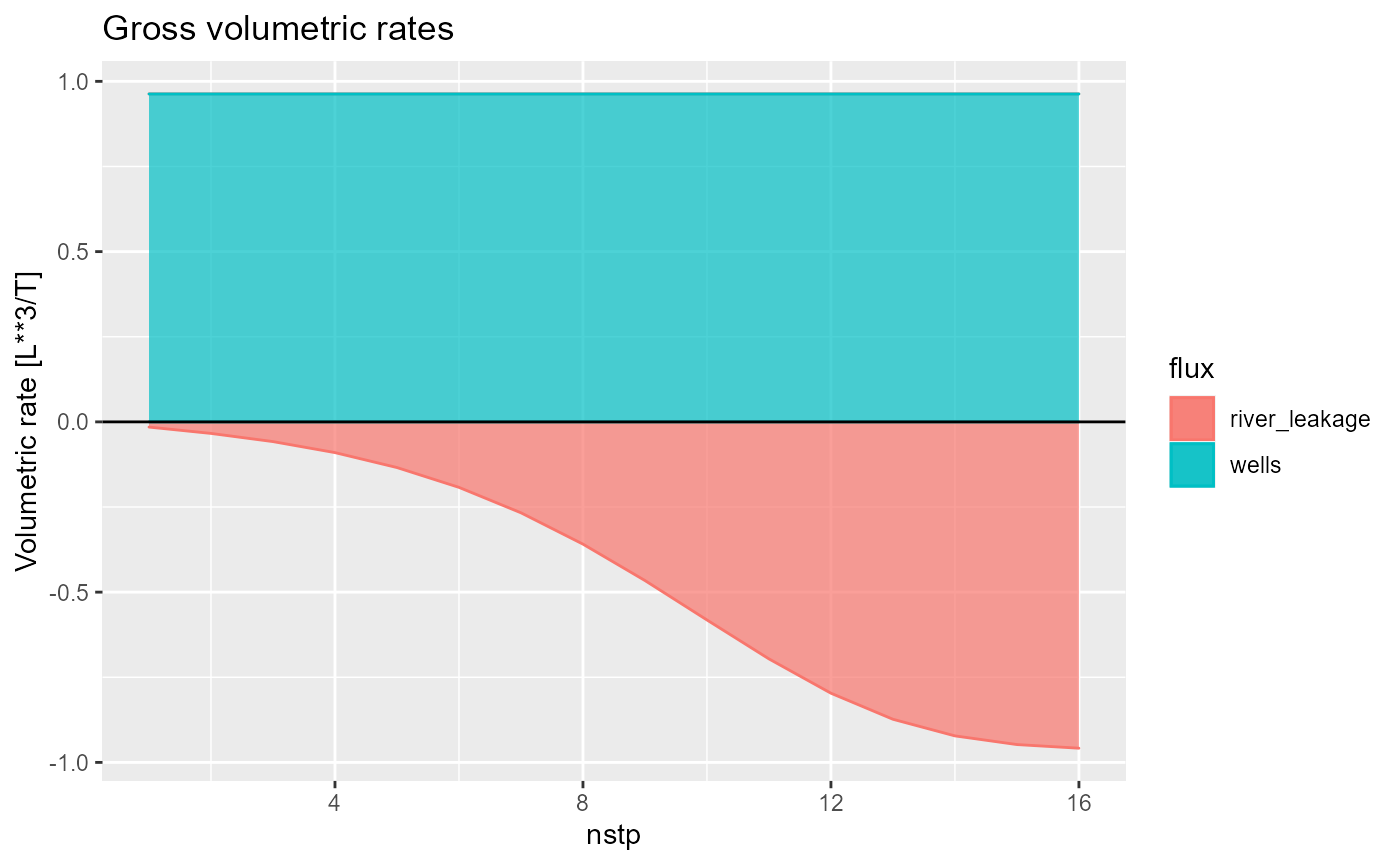
#> - attr(*, "class")= chr "bud"Plotting a bud object can be done with rmf_plot.bud() which by default plots gross volumetric rates for all fluxes:
rmf_plot(bud, dis = dis)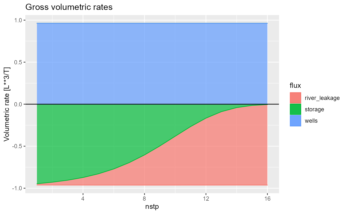
You can select fluxes with the fluxes argument,
plot net fluxes by setting net = TRUE
rmf_plot(bud, dis = dis, net = TRUE)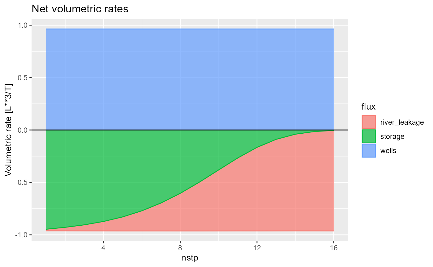
and select between rates, cumulative, total, difference or discrepancy using the what argument.
rmf_plot(bud, dis = dis, what = "cumulative")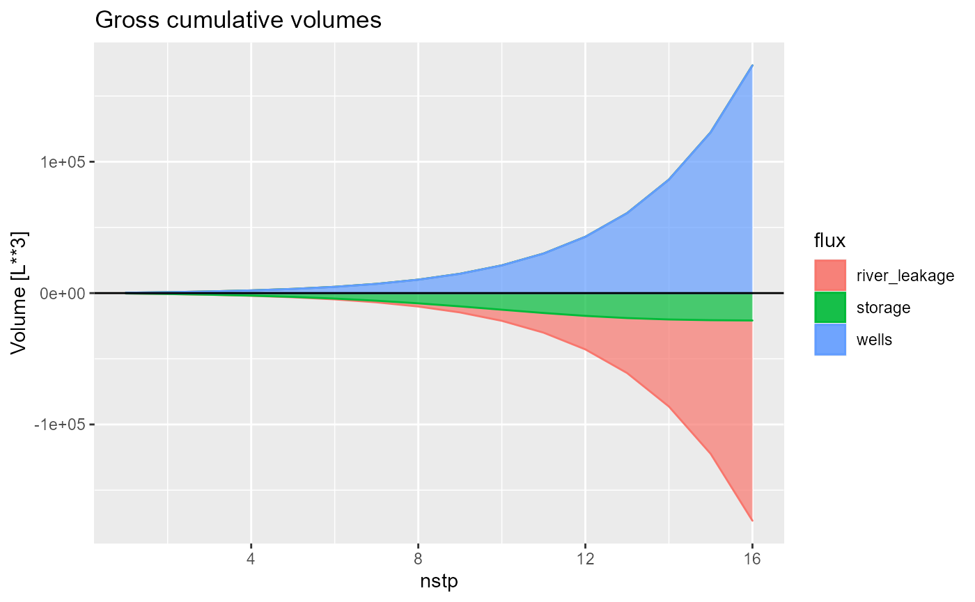
rmf_plot(bud, dis = dis, what = "discrepancy")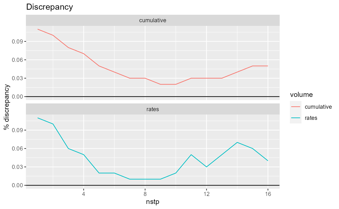
By default, rmf_plot.bud uses ggplot2::geom_area. You can change this to a bar plot (ggplot2::geom_col) by setting type = 'bar':
rmf_plot(bud, dis = dis, type = "bar")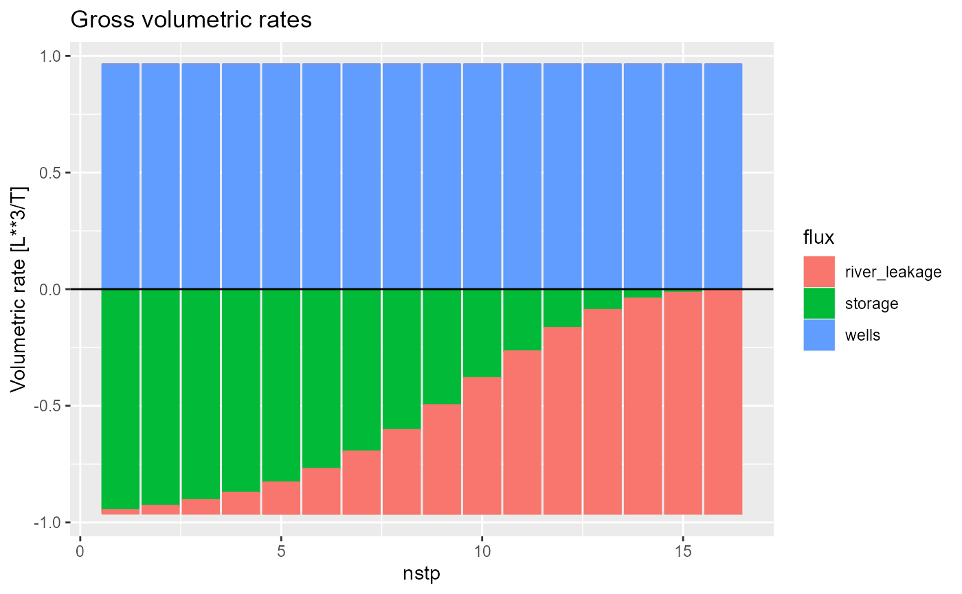
this is especially useful when plotting only a few time steps:
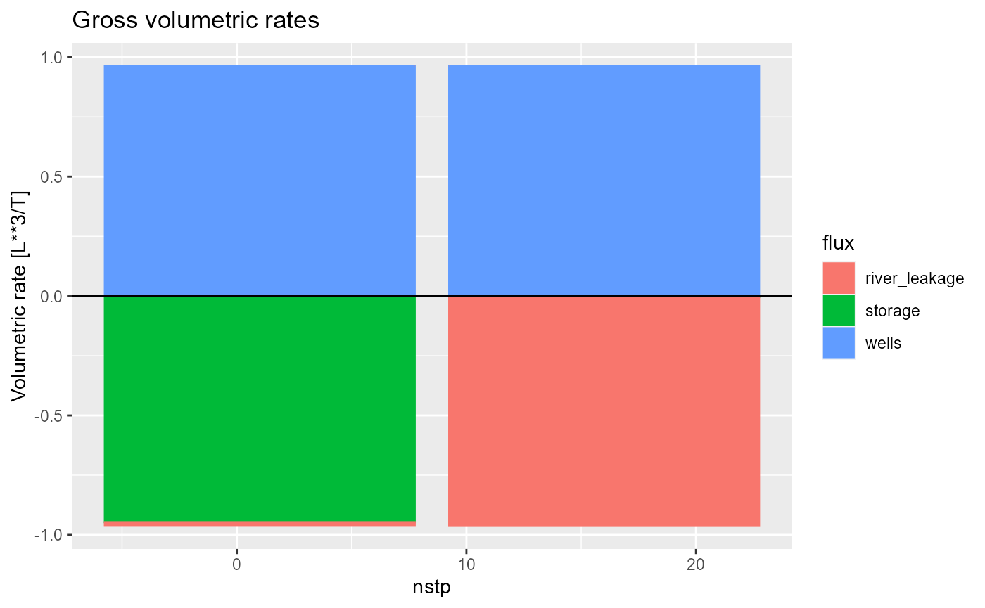
and is the default if the simulation only has a single time step (e.g. a steady-state simulation):
dis_ss <- rmf_example_file("example-model.dis") %>%
  rmf_read_dis()
bud_ss <- rmf_example_file("example-model.lst") %>%
  rmf_read_bud()

rmf_plot(bud_ss, dis = dis_ss)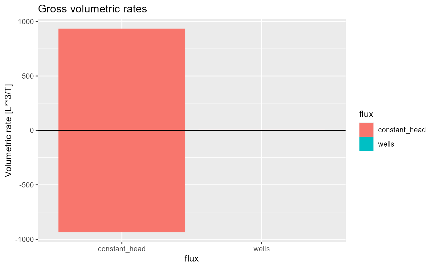
Head-prediction file
If a HOB file is present with a IUHOBS value larger than zero, a head-prediction file will be saved to disk by the MODFLOW simulation. This file holds the observed hydraulic head values, their simulated equivalents and the observation names. It can be read by RMODFLOW using rmf_read_hpr() which returns a data.frame of class hpr:
hpr <- rmf_example_file("water-supply-problem.hob_out") %>%
  rmf_read_hpr()
str(hpr)
#> Classes 'hpr' and 'data.frame':  27 obs. of  4 variables:
#>  $ simulated: num  0.0716 0.0716 0.0992 0.1844 0.2971 ...
#>  $ observed : num  0.17 0.26 0.33 0.48 0.57 ...
#>  $ name     : chr  "ObsWell1__1" "ObsWell1__2" "ObsWell1__3" "ObsWell1__4" ...
#>  $ residual : num  -0.0984 -0.1884 -0.2308 -0.2956 -0.2729 ...
rmf_read_hpr adds a residual column which is the difference between simulated and observed values.
To plot a hpr object, you can use rmf_plot.hpr() which by default plots a scatter plot:
rmf_plot(hpr)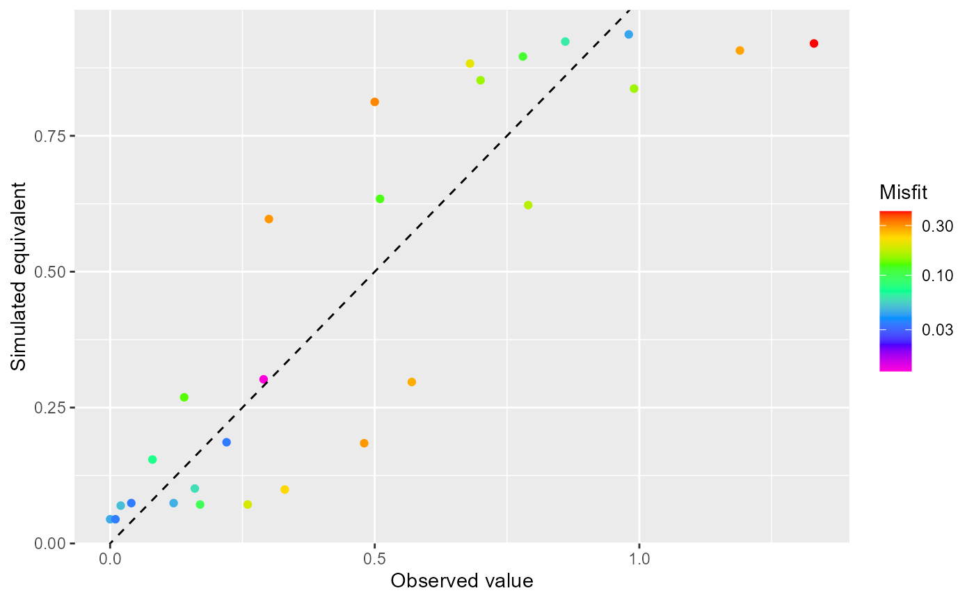
A histogram or residual plot can be made by changing the type argument:
rmf_plot(hpr, type = "histogram")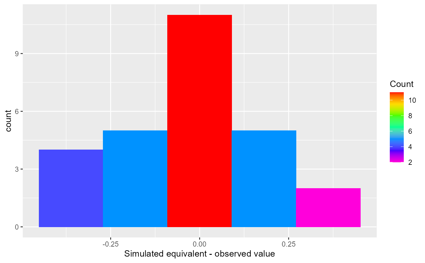
rmf_plot(hpr, type = "residual") + ggplot2::theme(axis.text.x.bottom = ggplot2::element_text(angle = 90))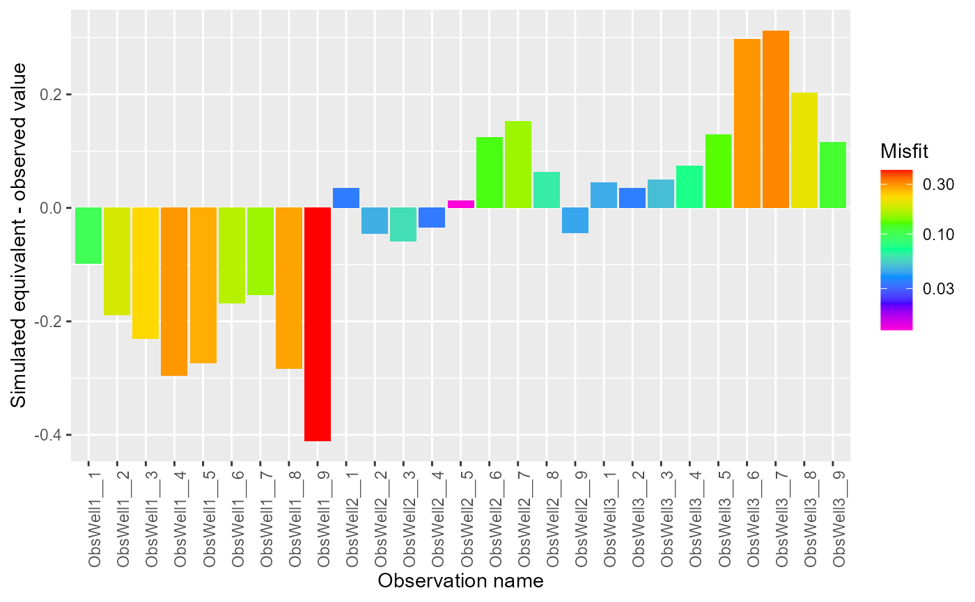
Goodness-of-fit statistics can be obtained with the rmf_performance() function:
rmf_performance(hpr)
#> Warning: 'rNSE' can not be computed: some elements in 'obs' are zero !
#> Warning: 'rd' can not be computed: some elements in 'obs' are zero !
#>      me  mae  mse rmse pbias  nse   r2  kge  ssq
#> 1 -0.02 0.15 0.03 0.18  -5.1 0.77 0.78 0.86 0.88
Output-Control
In MODFLOW, the Output-Control file (OC) controls the type and timing of saving output to disk and printing output to the listing file. RMODFLOW can read, write and create an OC object.
oc <- rmf_example_file("water-supply-problem.oc") %>%
  rmf_read_oc(dis = dis)
str(oc)
#> List of 22
#>  $ ibouun        : logi NA
#>  $ cboufm        : logi NA
#>  $ iddnun        : num 38
#>  $ cddnfm        : chr "(10(1X1PE13.5))"
#>  $ iddnfm        : logi NA
#>  $ ihedun        : num 37
#>  $ chedfm        : chr "(10(1X1PE13.5))"
#>  $ ihedfm        : logi NA
#>  $ ibound_label  : logi FALSE
#>  $ drawdown_label: logi TRUE
#>  $ head_label    : logi TRUE
#>  $ aux           : logi TRUE
#>  $ compact_budget: logi TRUE
#>  $ print_head    : logi [1:16] FALSE FALSE FALSE FALSE FALSE FALSE ...
#>  $ print_drawdown: logi [1:16] FALSE FALSE FALSE FALSE FALSE FALSE ...
#>  $ save_head     : logi [1:16] TRUE TRUE TRUE TRUE TRUE TRUE ...
#>  $ save_drawdown : logi [1:16] TRUE TRUE TRUE TRUE TRUE TRUE ...
#>  $ save_ibound   : logi [1:16] FALSE FALSE FALSE FALSE FALSE FALSE ...
#>  $ iperoc        : num [1:16] 1 1 1 1 1 1 1 1 1 1 ...
#>  $ itsoc         : num [1:16] 1 2 3 4 5 6 7 8 9 10 ...
#>  $ save_budget   : logi [1:16] TRUE TRUE TRUE TRUE TRUE TRUE ...
#>  $ print_budget  : logi [1:16] TRUE TRUE TRUE TRUE TRUE TRUE ...
#>  - attr(*, "comment")= chr " Output Control file created on 2017-05-30 by ModelMuse version 3.9.0.0."
#>  - attr(*, "class")= chr [1:2] "oc" "rmf_package"
When creating an OC object, you might be overwhelmed by the amount of input arguments. This is in large part because a MODFLOW OC file can be specified in two ways: either with words or numeric codes. RMODFLOW keeps true to these options but uses words by default.
The OC object controls saving of following variables to disk: head, drawdown, ibound & cell-by-cell-flows. It also controls the printing of following variables to the listing file: head, drawdown & volumetric budget.
By default, an OC object created by RMODFLOW specifies the following:
- Save heads at every time step
- Save cell-by-cell flows at every time step
- Print the volumetric budget to the listing file at every time step
- The head file is specified as binary
- Labels are written to the corresponding output files
- The compact budget option for the cbc file is active
- The aux option for compact budget is active
Remember that the cbc file is always binary.
To alter any of these, use the respective save_* or print_* arguments. These are logical values, either of length 1 meaning they are the same for all time steps, or a single value for every time step.
rmf_create_oc(dis = dis, print_head = TRUE,
              save_head = c(rep(FALSE, sum(dis$nstp)/2), rep(TRUE, sum(dis$nstp)/2) )) %>%
  str()
#> List of 22
#>  $ ihedfm        : num 0
#>  $ chedfm        : logi NA
#>  $ ihedun        : num 666
#>  $ iddnfm        : logi NA
#>  $ cddnfm        : logi NA
#>  $ iddnun        : logi NA
#>  $ cboufm        : logi NA
#>  $ ibouun        : logi NA
#>  $ compact_budget: logi TRUE
#>  $ aux           : logi TRUE
#>  $ head_label    : logi TRUE
#>  $ drawdown_label: logi TRUE
#>  $ ibound_label  : logi TRUE
#>  $ iperoc        : int [1:16] 1 1 1 1 1 1 1 1 1 1 ...
#>  $ itsoc         : int [1:16] 1 2 3 4 5 6 7 8 9 10 ...
#>  $ print_head    : logi [1:16] TRUE TRUE TRUE TRUE TRUE TRUE ...
#>  $ print_drawdown: logi [1:16] FALSE FALSE FALSE FALSE FALSE FALSE ...
#>  $ print_budget  : logi [1:16] TRUE TRUE TRUE TRUE TRUE TRUE ...
#>  $ save_head     : logi [1:16] FALSE FALSE FALSE FALSE FALSE FALSE ...
#>  $ save_drawdown : logi [1:16] FALSE FALSE FALSE FALSE FALSE FALSE ...
#>  $ save_ibound   : logi [1:16] FALSE FALSE FALSE FALSE FALSE FALSE ...
#>  $ save_budget   : logi [1:16] TRUE TRUE TRUE TRUE TRUE TRUE ...
#>  - attr(*, "class")= chr [1:2] "oc" "rmf_package"
To set the unit numbers on which the output is saved, use the ihedun (default 666), iddnun (default 667) & ibouun (default 668) values for heads, drawdowns and ibound output, respectively. The unit number for cell-by-cell flows is set in the flow and boundary condition packages.
rmf_create_oc(dis = dis,
              ihedun = 50,
              save_drawdown = TRUE, iddnun = 60) %>%
  str()
#> List of 22
#>  $ ihedfm        : logi NA
#>  $ chedfm        : logi NA
#>  $ ihedun        : num 50
#>  $ iddnfm        : logi NA
#>  $ cddnfm        : logi NA
#>  $ iddnun        : num 60
#>  $ cboufm        : logi NA
#>  $ ibouun        : logi NA
#>  $ compact_budget: logi TRUE
#>  $ aux           : logi TRUE
#>  $ head_label    : logi TRUE
#>  $ drawdown_label: logi TRUE
#>  $ ibound_label  : logi TRUE
#>  $ iperoc        : int [1:16] 1 1 1 1 1 1 1 1 1 1 ...
#>  $ itsoc         : int [1:16] 1 2 3 4 5 6 7 8 9 10 ...
#>  $ print_head    : logi [1:16] FALSE FALSE FALSE FALSE FALSE FALSE ...
#>  $ print_drawdown: logi [1:16] FALSE FALSE FALSE FALSE FALSE FALSE ...
#>  $ print_budget  : logi [1:16] TRUE TRUE TRUE TRUE TRUE TRUE ...
#>  $ save_head     : logi [1:16] TRUE TRUE TRUE TRUE TRUE TRUE ...
#>  $ save_drawdown : logi [1:16] TRUE TRUE TRUE TRUE TRUE TRUE ...
#>  $ save_ibound   : logi [1:16] FALSE FALSE FALSE FALSE FALSE FALSE ...
#>  $ save_budget   : logi [1:16] TRUE TRUE TRUE TRUE TRUE TRUE ...
#>  - attr(*, "class")= chr [1:2] "oc" "rmf_package"
To save ASCII files, set the chedfm, cddnfm or cboufm values to proper FORTRAN formats enclosed in parenthesis containing no more than 20 characters. These FORTRAN formats can be found in the MODFLOW-2005 manual. In RMODFLOW, you can alternatively specify integer codes for the save formats, similar to the print formats. RMODFLOW will convert these to the proper FORTRAN format. Note that ASCII files are typically larger than binary files.
rmf_create_oc(dis = dis, chedfm = 0) %>%
  str()
#> List of 22
#>  $ ihedfm        : logi NA
#>  $ chedfm        : chr "(10G11.4)"
#>  $ ihedun        : num 666
#>  $ iddnfm        : logi NA
#>  $ cddnfm        : logi NA
#>  $ iddnun        : logi NA
#>  $ cboufm        : logi NA
#>  $ ibouun        : logi NA
#>  $ compact_budget: logi TRUE
#>  $ aux           : logi TRUE
#>  $ head_label    : logi TRUE
#>  $ drawdown_label: logi TRUE
#>  $ ibound_label  : logi TRUE
#>  $ iperoc        : int [1:16] 1 1 1 1 1 1 1 1 1 1 ...
#>  $ itsoc         : int [1:16] 1 2 3 4 5 6 7 8 9 10 ...
#>  $ print_head    : logi [1:16] FALSE FALSE FALSE FALSE FALSE FALSE ...
#>  $ print_drawdown: logi [1:16] FALSE FALSE FALSE FALSE FALSE FALSE ...
#>  $ print_budget  : logi [1:16] TRUE TRUE TRUE TRUE TRUE TRUE ...
#>  $ save_head     : logi [1:16] TRUE TRUE TRUE TRUE TRUE TRUE ...
#>  $ save_drawdown : logi [1:16] FALSE FALSE FALSE FALSE FALSE FALSE ...
#>  $ save_ibound   : logi [1:16] FALSE FALSE FALSE FALSE FALSE FALSE ...
#>  $ save_budget   : logi [1:16] TRUE TRUE TRUE TRUE TRUE TRUE ...
#>  - attr(*, "class")= chr [1:2] "oc" "rmf_package"
Let’s say, we want to save drawdowns in an ASCII file (setting cddnfm to a FORTRAN format or positive integer) on unit number 50 (default is 667 for drawdown), not save heads, and print volumetric budget to the listing file every other time step:
oc <- rmf_create_oc(dis = dis,
                    save_drawdown = TRUE, cddnfm = 0, iddnun = 50,
                    save_head = FALSE,
                    print_budget = rep(c(FALSE, TRUE), sum(dis$nstp)/2))
str(oc)
#> List of 22
#>  $ ihedfm        : logi NA
#>  $ chedfm        : logi NA
#>  $ ihedun        : logi NA
#>  $ iddnfm        : logi NA
#>  $ cddnfm        : chr "(10G11.4)"
#>  $ iddnun        : num 50
#>  $ cboufm        : logi NA
#>  $ ibouun        : logi NA
#>  $ compact_budget: logi TRUE
#>  $ aux           : logi TRUE
#>  $ head_label    : logi TRUE
#>  $ drawdown_label: logi TRUE
#>  $ ibound_label  : logi TRUE
#>  $ iperoc        : int [1:16] 1 1 1 1 1 1 1 1 1 1 ...
#>  $ itsoc         : int [1:16] 1 2 3 4 5 6 7 8 9 10 ...
#>  $ print_head    : logi [1:16] FALSE FALSE FALSE FALSE FALSE FALSE ...
#>  $ print_drawdown: logi [1:16] FALSE FALSE FALSE FALSE FALSE FALSE ...
#>  $ print_budget  : logi [1:16] FALSE TRUE FALSE TRUE FALSE TRUE ...
#>  $ save_head     : logi [1:16] FALSE FALSE FALSE FALSE FALSE FALSE ...
#>  $ save_drawdown : logi [1:16] TRUE TRUE TRUE TRUE TRUE TRUE ...
#>  $ save_ibound   : logi [1:16] FALSE FALSE FALSE FALSE FALSE FALSE ...
#>  $ save_budget   : logi [1:16] TRUE TRUE TRUE TRUE TRUE TRUE ...
#>  - attr(*, "class")= chr [1:2] "oc" "rmf_package"